Reproducing analysis on wine data
Rani Basna
2021-09-17
Source:vignettes/DKK_and_Functional_analysis_on_wine_data.Rmd
DKK_and_Functional_analysis_on_wine_data.RmdThis article attempts at reproducing the results presented at the paper Machine Learning Assisted Orthonormal Basis Selection for Functional Data Analysis.
Libraies
# install.packages("Splinets") for Orthogonal projections
library(Splinets)
library(DDK)
library(ggplot2)
library(reshape2)
library(RColorBrewer)
We will first write few helper functions. These functions depends on few packages. Most importantly, the package Splinets. In order to get a full understanding of these objects and functions, one needs some understanding of the DDK methods presented in above mentioned paper as well as the practicle usage of the package Splinets presented at this arxiv paper
Helper Functions
# function that helps in plotting the functional data
df_plot_fda <- function(S_data, time_df, s=1, a= 0.8, n_sample = 10){
  # to do
  # check that the length of the time data agree with the dim of the data
  # write an if statment that in case of empty time_df generate a one based on the dim S_data
  df_plot <- as.data.frame(t(S_data))
  # selecting samples
  df_plot_n <- df_plot[,1:n_sample]
  # add the time var
  df_plot_n$time <- time_df
  df_plot_melt_n <- melt(df_plot_n, id.vars=c("time"))
  # ploting
  plot_n <- ggplot(df_plot_melt_n, aes(x=time, y = value, color=variable)) + geom_line(size=s, alpha=a) + theme_minimal() + theme(legend.position = "none", axis.title = element_blank(), axis.text.y = element_blank())
  res <- list(plot_n, df_plot_melt_n)
  return(res)
}
# prepare the data
data_prepare <- function(f_data, t_data){
        colnames(f_data) <- NULL
        colnames(t_data) <- NULL
        f_data <- t(f_data)
        ready_data <- cbind(t_data, f_data)
        ready_data <- as.matrix(ready_data)
        return(ready_data)
}
# Prepare knots
Knots_prepare <- function(selected_knots, Time){
        knots_normalized <- selected_knots / max(selected_knots)
        knots_normalized = knots_normalized*(max(Time)- min(Time)) + min(Time)
        # taking the first three decimal number
        knots_normalized = as.numeric(format(round(knots_normalized,4), nsmall = 1))
        return(knots_normalized)
}
#
GetProjCovEig <- function(f_ready_data, ready_knots){
  ProjObj <- project(f_ready_data,ready_knots)
  Sigma=cov(ProjObj$coeff)
  Spect=eigen(Sigma,symmetric = T)
  EigenSp=lincomb(ProjObj$basis,t(Spect$vec))
  Proj_C_EV <- list(ProjObj = ProjObj, Sigma=Sigma, Spect=Spect, EigenSp=EigenSp)
  return(Proj_C_EV)
}
#
compare_fit <- function(N_plots, SubsampleFractions, ProjCovEigObj){
  if(!is.vector(SubsampleFractions)){
    stop("SubsampleFractions has to be a vector of subsamples")
  }
  if(!(length(SubsampleFractions) == N_plots)){
    stop("length of SubsampleFractions has to be equal to the N_plots")
  }
  EgnFncts <- list()
  for(i in 1:N_plots){
    EgnFncts[i] = subsample(ProjCovEigObj$EigenSp,1:SubsampleFractions[i])
  }
  return(EgnFncts)
}
#
get_Compare_Plot <- function(ready_f_data, ProjCovEigObj, portions = c(), EgnFuncObj, sampleNumber){
  C_mat=ProjCovEigObj$ProjObj$coeff %*% ProjCovEigObj$Spect$vec
    return({matplot(ready_f_data[,1],ready_f_data[,sampleNumber],type='l',lty=1,xlab='',ylab='')
            lines(ProjCovEigObj$ProjObj$sp,sID=sampleNumber-1,col='red',lty=2,lwd=1)
            if(length(portions > 0)){
             lines(lincomb(EgnFuncObj[[1]],C_mat[1,1:portions[1],drop=F]),col='green')
             lines(lincomb(EgnFuncObj[[2]],C_mat[1,1:portions[2],drop=F]),col='brown')
             lines(lincomb(EgnFuncObj[[3]],C_mat[1,1:portions[3],drop=F]),col='blue',lwd=1)}
             })
}
#
get_amse_diff <- function(f_ready_data, ProjCovEigObj, t_data){
  if(is.data.frame(t_data)){
    f_hat <- evspline(object = ProjCovEigObj$ProjObj$sp, x = t_data[,1])
  }
  if(is.vector(t_data)){
    f_hat <- evspline(object = ProjCovEigObj$ProjObj$sp, x = t_data)
  }
  f_diff <- f_hat - f_ready_data
  AMSE_diff <- dim(f_ready_data)[1] * amse(f_diff[,-1])
  # AMSE_diff <- amse(f_diff[,-1])
  AMSE_diff_list = list(f_hat, f_diff, AMSE_diff)
  return(AMSE_diff_list)
}
#
plot_EigenfunctionEigenValueScaled <- function(ProjCovEigObj, EigenNumber, mrgn=2, type='l', bty="n",col='deepskyblue4',
                       lty=1, lwd=2, xlim=NULL, ylim = NULL, xlab="", ylab = "", vknots=TRUE){
  if(!is.numeric(EigenNumber)){
    stop(" please insert the number of eigenfunctions as EigenMuber")
  }
  y = evspline(ProjCovEigObj$EigenSp, sID = 1:EigenNumber)
  Arg=y[,1]
  Val=y[,-1,drop=F]
  # if(is.null(xlim)){
  #   xlim = range(Arg)
  # }
  # if(is.null(ylim)){
  #   ylim = range(Val)
  # }
  plot(Arg,Val[,1]*sqrt(ProjCovEigObj$Spect$values[1]),type=type,bty=bty,col=col,xlim=xlim,ylim=ylim,
       xlab=xlab,ylab=ylab,lty=lty,lwd=lwd)
  ourcol=c( 'darkorange3', 'goldenrod', 'darkorchid4',
              'darkolivegreen4', 'deepskyblue', 'red4',
              'slateblue','deepskyblue4')
  for(i in 2:EigenNumber){
      lines(Arg,Val[,i]*sqrt(ProjCovEigObj$Spect$values[i]),col=ourcol[(i-2)%%8+1],lty=lty,lwd=lwd)
  }
  if(vknots){
    abline(v = ProjCovEigObj$EigenSp@knots, lty = 3, lwd = 0.5)
  }
  abline(h = 0, lwd = 0.5)
}
wine data
For more details on the wine data, see the description part of the data in the DDK paper.
# get the data from the DKK pacakge
data("Wine")
f_data_wine <- Wine$x.learning
t_df_wine <- seq(1, dim(f_data_wine)[2])
# test data
f_data_wine_test <- Wine$x.test
t_df_wine_test <- seq(1, dim(f_data_wine_test)[2])
# remove raw 84 since it is an outlier
f_data_wine <- f_data_wine[-84,]
# ploting
wine_plot <- df_plot_fda(S_data = f_data_wine, time_df = t_df_wine, a = 1, s = 0.5, n_sample = 10)
p <- wine_plot[[1]]
p <- p + scale_color_brewer(palette = "PuOr")  + theme(legend.position = "None")
p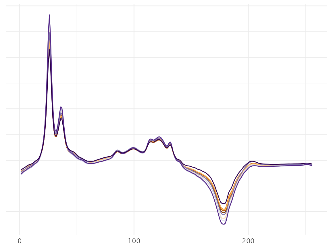
Next, we run the DKK algorithm using the add_knots function. We need to input the training data, the test data, the search for the knots interval as well as the requested number of knots.
# knot selection
initial_knots <- c(0, dim(f_data_wine)[2])
initial_knots
#> [1] 0 256
# selecting the knots with add_knots function
KS_wine <- add_knots(f = f_data_wine, f_v = f_data_wine_test, knots = initial_knots, L = 8, M = 1)
#> proposed splits is 139
#> proposed splits is 40 193
#> [1] "printing the new knot"
#> [1] 139
#> current TMSE is 0.004905913
#> proposed splits is 40 167 199
#> [1] "printing the new knot"
#> [1] 193
#> current TMSE is 0.004905913 0.004309568
#> proposed splits is 40 154 186 199
#> [1] "printing the new knot"
#> [1] 167
#> current TMSE is 0.004905913 0.004309568 0.00378134
#> proposed splits is 21 83 154 186 199
#> [1] "printing the new knot"
#> [1] 40
#> current TMSE is 0.004905913 0.004309568 0.00378134 0.003386486
#> proposed splits is 15 28 83 154 186 199
#> [1] "printing the new knot"
#> [1] 21
#> current TMSE is 0.004905913 0.004309568 0.00378134 0.003386486 0.001677066
#> proposed splits is 15 NA 34 83 154 186 199
#> [1] "printing the new knot"
#> [1] 28
#> current TMSE is 0.004905913 0.004309568 0.00378134 0.003386486 0.001677066 0.001368651
#> proposed splits is 15 NA 34 83 154 173 NA 199
#> [1] "printing the new knot"
#> [1] 186
#> current TMSE is 0.004905913 0.004309568 0.00378134 0.003386486 0.001677066 0.001368651 0.001266586
#> proposed splits is 15 NA 34 48 133 154 173 NA 199
#> [1] "printing the new knot"
#> [1] 83
#> current TMSE is 0.004905913 0.004309568 0.00378134 0.003386486 0.001677066 0.001368651 0.001266586 0.00116028
KS_wine$Fknots
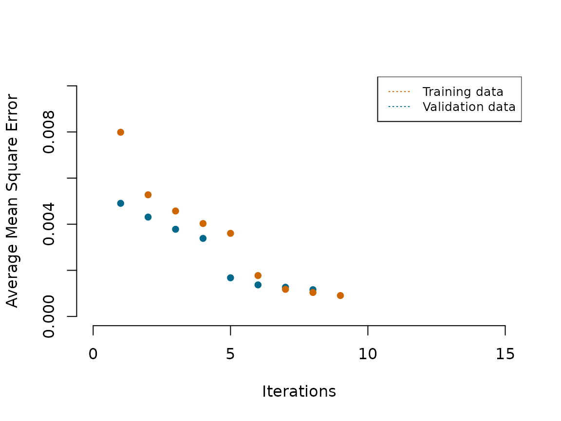
#> [1] 0 21 28 40 83 139 167 186 193 256Next, we plot the reduction in AMSE in the Functional Wine data.(Orange-bottom) reduction in AMSE achieved after each additional knot selection during training.(Blue-top) reduction achieved after each additional knot selection on the validation data.
# ploting the reduction of the AMSE
# For train data
df_knots_wine <- data.frame("x" = seq_len(length(KS_wine[[3]])), "Error_reduction" = KS_wine[[3]])
# For test data
df_knots_wine_test <- data.frame("x" = seq_len(length(KS_wine[[4]])), "Error_reduction" = KS_wine[[4]])
# ploting amse reduction
{plot(x =  df_knots_wine_test$x,y =  df_knots_wine_test$Error_reduction,type='p',pch=16, xlim = c(0,15), ylim = c(0,0.01),ylab='Average Mean Square Error',xlab='Iterations', bty="n", col="deepskyblue4")
lines(x =  df_knots_wine$x,y= df_knots_wine$Error_reduction,type='p', pch=16, col='darkorange3')
legend("topright", legend = c("Training data", "Validation data"),
  col = c("darkorange3", "deepskyblue4"), lty = 3:3, cex = 0.8)
}
Let us plot the data with the selected knots to visualize how the DDK algorithm chooses the knots locations. This figure displays the outcome of the validation process and the selected knots from the training and validations represented in dashed lines.
# ploting
plot_dist_knots_wine <- df_plot_fda(S_data = f_data_wine, time_df = t_df_wine)
plot_dist_knots_wine[[1]]  + geom_vline(xintercept = KS_wine[[1]], linetype="dotted") + scale_color_brewer(palette = "PuOr")  + theme(legend.position = "None")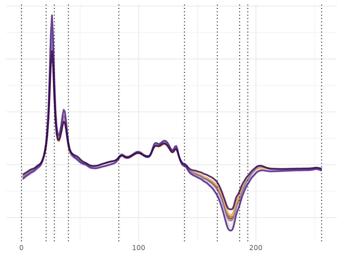
Comparing equidistance to the knote selection method
We first start by defining some needed objects. For more details on these objects see the package Splinets
Wine_DDKnots <- Knots_prepare(selected_knots = KS_wine[[1]], Time = t_df_wine)
n = length(Wine_DDKnots) - 1Knot_selection DKK case
Wine_DDKnots <- Knots_prepare(selected_knots = KS_wine[[1]], Time = t_df_wine)
WineObj <- GetProjCovEig(f_ready_data = Wine_prepared, ready_knots = Wine_DDKnots)
We first plot the eigenvalues ordered in a decreasing manner
plot(WineObj$Spect$values, type ='p',col='darkorange3', lwd=4, ylab="", xlab="", bty="n")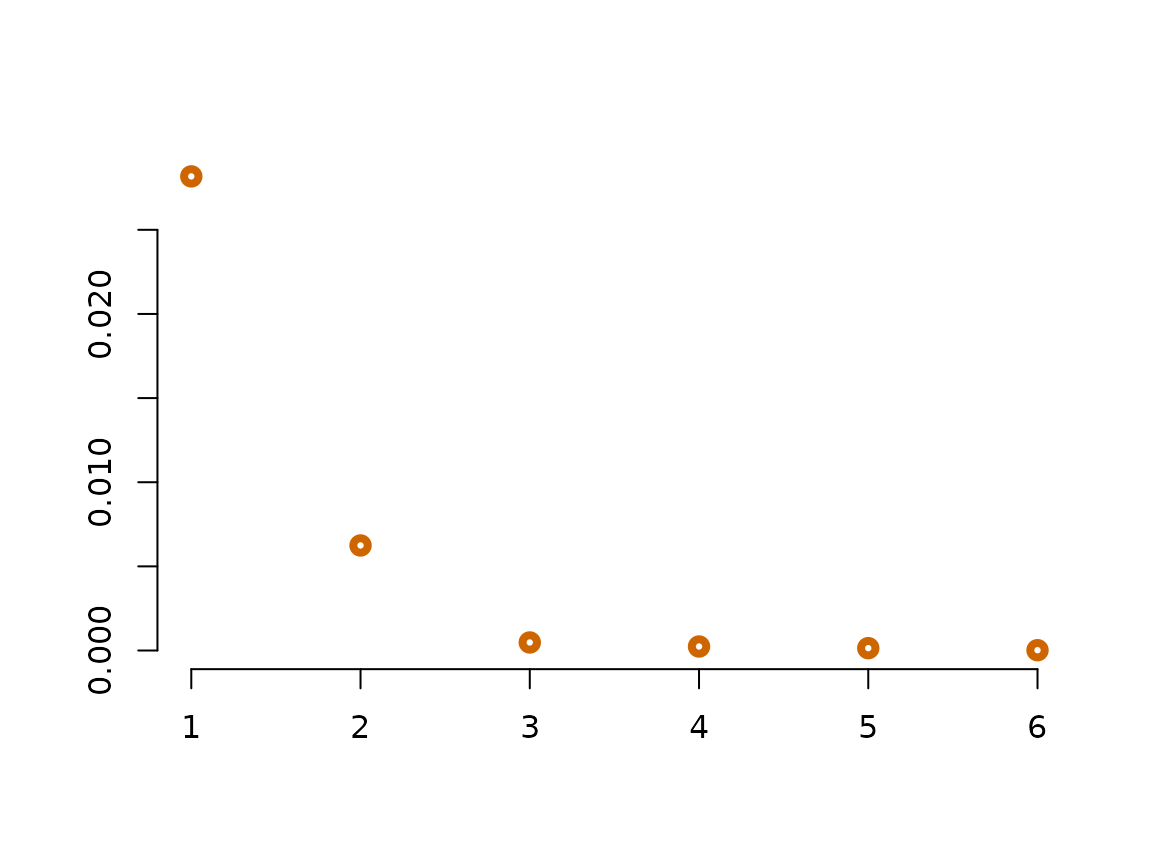
Next, we plot the first three eigen functions scaled by the square roots of their corresponding eigenvalues.
plot_EigenfunctionEigenValueScaled(ProjCovEigObj = WineObj, EigenNumber = 3) 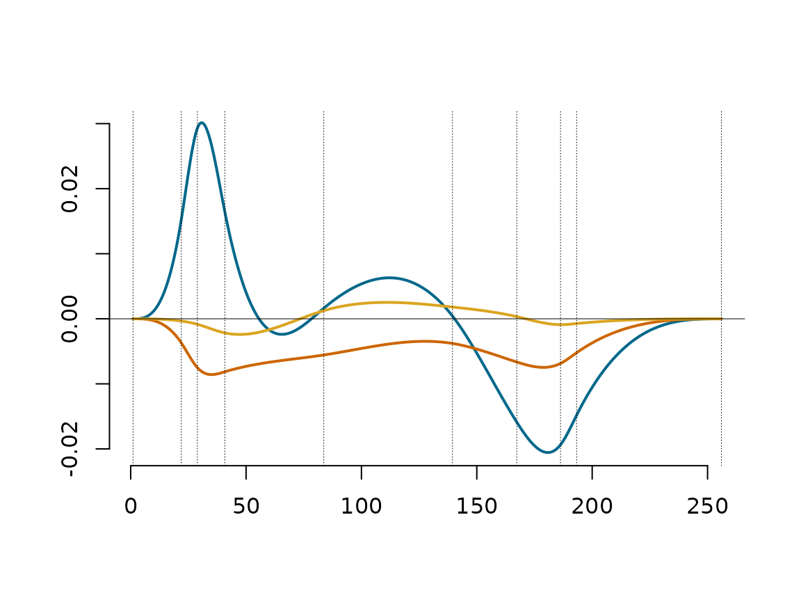
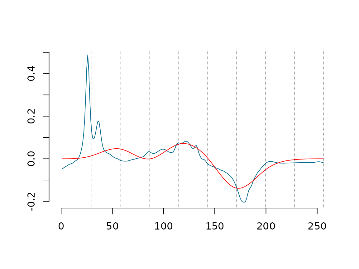
Next figure, One sample data (Blue curve), the projected data into splinets build over the knots chosen with DDK(yellow curve) with the location of the selected knots (vertical dashed lines), and the data decomposed using only the first eigenfunctions(orange curve);
C_mat_Wine=WineObj$ProjObj$coeff %*% WineObj$Spect$vec
EgenFunWine1 <- subsample(WineObj$EigenSp, 1)
{matplot(Wine_prepared[,1],Wine_prepared[,2],type='l',lty=1,xlab='',ylab='', bty="n",
         col="deepskyblue4", xlim = c(-1.5,dim(f_data_wine)[2]))
             lines(WineObj$ProjObj$sp,sID=2-1,col='goldenrod',lty=1,lwd=1)
             lines(lincomb(EgenFunWine1,C_mat_Wine[1,1,drop=F]),col='darkorange3')
             abline(v = WineObj$EigenSp@knots, lty = 3, lwd = 0.5)}
Finally, One sample data (Blue curve), the projected data into splinets build over equally spaced knots (yellow curve)with the location of the knots (vertical dashed lines).
{matplot(Wine_prepared[,1],Wine_prepared[,2],type='l',lty=1,xlab='',ylab='', bty="n",
         col="deepskyblue4", xlim = c(-1.5,dim(f_data_wine)[2]))
             # the equi distance
             lines(WineObj_eqi$ProjObj$sp, sID=2-1, col='red', lty=1,lwd=1)
             abline(v = WineObj_eqi$EigenSp@knots, lty = 3, lwd = 0.5)}